An Experiment for Factors Influencing Mung Beans Sprouting Speed
Xiaotian Wang
Graduate Student
Department of Statistics, University of Wisconsin Madison
Course Project for STAT 602: Statistical Method II
May 5th, 2020
Abstract
In this work, 4 factors influencing mung beans sprouting speed are considered. These factors are temperature, impurity level of water, soaking time, and watering frequency respectively. A 2n factorial experiment is designed to detect all possible significant effects. A preliminary experiment with no replicate and a formal experiment with 8 replicates are performed. To analyze the result of the preliminary experiment, neglecting high order interaction method, Loh��s method, Lenth��s method and Dong��s method are used. Together with the formal experiment, we construct the 90% and 95% simultaneous confidence interval and manage to find the significant effects. Additionally, the interpretations are also been made.
Keywords: Mung bean sprout, design of experiment, factorial design, 2n design, ANOVA, Loh��s method, Lenth��s method, Dong��s method
An Experiment for Factors Influencing Mung Beans Sprouting Speed
Mung bean sprouts are a kind of vegetable consumed mainly in East Asia grown by sprouting mung beans. Generally, there are two class of methods to sprout the mung beans: one for commercial use and the other for home use. For home use methods, they can be grown by placing and watering the sprouted beans in the shade until the roots grow long. Here, we only focus on the home-used method: only by watering the mung beans to sprout them instead of using soil.
There are many factors that can influence the speed that mung beans sprout. We are interested in the problem that under what conditions the mung bean sprouts can grow faster. After exploring this, we can draw some conclusions that can help us to sprout the mung beans faster. In this project, we only focus on the following four factors that may influence the growing speed: (A)temperature, (B) impurities level of water, (C)time we soak the mung beans in water and, (D)frequencies we sprinkle water on the mung beans. We will discuss about these factors in details in the following sections.
1 Design of Experiment
We designed a completely randomized 24 factorial design with two levels to explore the factors influencing mung beans sprouting speed. The details of the design are introduced in this section.
1. 1 Experimental Procedure
To make the mung beans sprout and grow, we first need to soak the mung beans in water for some time (factor C) to wake mung beans up and to make the mung beans begin to sprout. To do this, we plan to use small plastic cups(2oz) with water in it to soak the mung beans for some time. Then, we punch some holes at the bottom of the cup to let the water flow out. After that, we can sprinkle water on the mung beans every some time (factor D mentioned) to keep the mung beans wet and growing. For the whole process, we will try to make the mung
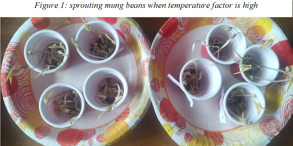 |
beans in a dark environment. Here is a photo of what the experiment is like. See figure 1 below:
1. 2 Variable and Factor Descriptions
Response Variable
With different factors, we sprout the mung beans in different ways but last for same time (5 days in total) and observe the length of the sprouts. We use the length(cm) to be the response variable in this experiment. The greater the value of the variable is, the faster the sprouts grow.
Factor A: Temperature
Temperature will influence the growth rate of plants. However, it also depends on the habits of the specific plant. We wish to see how higher and lower temperature will influence the growth rate of sprouts. We use the home temperature which is 25 Celsius for high factor level and fridge temperature which is 10 Celsius for low factor level.
Factor B: Impurities Level of Water
For each group, we use same kind of water to both soak and sprinkle on the mung beans.
As we know, there are different kind of impurities in the daily water for example microorganism and minerals (Ca2+, Mg2+, etc.). They may be the nutrition for mung beans to grow, but they may also restrain the growth of mung beans sprouts. So, we design the the factors to two levels: high and low to see how this factor influence the growth of mung beans growth.
For high level, we directly use the water from Lake Mendota. The lake water is considered to be full of natural impurities. For low level, we use the boiled water since we think most of the microorganism in water will be killed, and the minerals will precipitate as the form of limescale (CaCO3,Mg(OH)2,etc.) by boiling it.
Factor C: Soaking Time
We design the soaking time factors to be high (12 hours) and low (6 hours). If this factor is tested to be nonsignificant, we will know that it is unnecessary for us to soak the mung beans for too long time, which can improve our technics.
Factor D: Water Sprinkling Frequencies
We design the water sprinkling frequencies to be high (every 6 hours) and low (every 18 hours). If this factor is tested to be nonsignificant, we will know that it is unnecessary for us to sprinkle the water on the mung beans too frequently, which can save our time and water.
For a summary of factors, please refer table 1 below:
Table 1:Summary of Factors and Descriptions
|
Factors |
High Level (+) |
Low Level (-) |
|
A: Temperature |
25 Celsius |
10 Celsius |
|
B: Impurities Level of Water |
lake water |
boiled water |
|
C: Soaking Time |
12 hours |
6 hours |
|
D: Water Sprinkling Frequencies |
every 6 hours |
Every 18 hours |
1. 3 Preliminary Experiment and Formal Experiment
For the whole experiment, we design the preliminary experiment with unreplicated data and formal experiment with replicated data.
For preliminary experiment, considering that the sprouting rate is less than 100%, for each run, we use 5 mung beans at the beginning and when they sprout (some of them may not sprout), we randomly choose one sprouting as the observation.
Based on the experience of preliminary experiment, we can then perform the formal experiment. For each run of the formal experiments, we use 15 mung beans at the beginning and finally randomly choose 8 of the beans which have sprouted as the observations. The data from the preliminary experience will NOT be used in the formal experience. So, the number of replicates is 8.
2 Preliminary Experiment
We conduct a preliminary experiment with unreplicated data in order to provide some experience to the formal experiment. In this section, the data results and related data analysis are introduced.
2. 1 Data Presentation
After 5 days of preliminary experiment, we collect the data which are summarized in the following table 2:
Table 2: data presentation of preliminary experiment
|
B |
C |
D |
Response (cm) |
|
|
+ |
+ |
+ |
+ |
7.9 |
|
+ |
+ |
+ |
- |
4.2 |
|
+ |
+ |
- |
+ |
9.1 |
|
+ |
+ |
- |
- |
4.5 |
|
+ |
- |
+ |
+ |
8.9 |
|
+ |
- |
+ |
- |
7.2 |
|
+ |
- |
- |
+ |
9.2 |
|
+ |
- |
- |
- |
7.1 |
|
- |
+ |
+ |
+ |
3.0 |
|
- |
+ |
+ |
- |
1.8 |
|
- |
+ |
- |
+ |
3.4 |
|
- |
+ |
- |
- |
2.9 |
|
- |
- |
+ |
+ |
3.7 |
|
- |
- |
+ |
- |
5.1 |
|
- |
- |
- |
+ |
5.7 |
|
- |
- |
- |
- |
5.2 |
In this table, ��+�� means at high level and ��-�� means at low level.
2. 2 Analysis of Variance
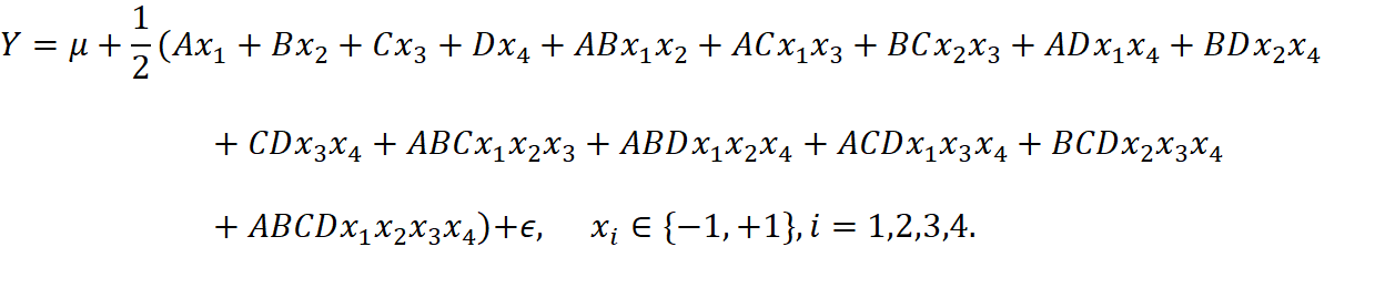
The full model we have is

and we need first compute the estimate of each effects. The results are shown in table 3:
Table 3: estimate of effects for preliminary experiment
|
Effects |
Estimate |
Effects |
Estimate |
|
A |
3.4125 |
BD |
0.8875 |
|
B |
-1.9125 |
CD |
-0.3125 |
|
C |
-0.6625 |
ABC |
-0.2375 |
|
D |
1.6125 |
ABD |
-0.2375 |
|
AB |
0.2375 |
ACD |
-0.0125 |
|
AC |
0.2375 |
BCD |
0.2625 |
|
BC |
-0.0875 |
ABCD |
-0.3875 |
|
AD |
1.4125 |
|
|
To
make any inference about the effect estimates, the ![]() must be estimated. In the
following subsections, inferences are made to detect any property of
significance.
must be estimated. In the
following subsections, inferences are made to detect any property of
significance.
2.2.1 Estimate  by Interactions
In this subsection, we assume some high order interactions to be negligible to estimate the variance by the average of the squares of these high-order interactions.
If the 4-factor interaction ABCD is assumed to be negligible, then we have
with degree of freedom 1(which is the number of effects we use to estimate the variance). Then, we can compute the simultaneous critical value
![]()
where ![]() is
the confidence level,
is
the confidence level, ![]() is the number of effects
we use to estimate the variance, and
is the number of effects
we use to estimate the variance, and ![]() is the number if effects
left. This simultaneous critical value means that if the abstract value of the effect
estimate is greater than the critical value, the simultaneous confidence
interval will not contain
is the number if effects
left. This simultaneous critical value means that if the abstract value of the effect
estimate is greater than the critical value, the simultaneous confidence
interval will not contain ![]() , and thus, the
corresponding effect will be significant at
, and thus, the
corresponding effect will be significant at ![]() level. We try to assume
different effects negligible to estimate the variance and get the following
table 4:
level. We try to assume
different effects negligible to estimate the variance and get the following
table 4:
Table 4: neglect high order interactions to estimate variance and detect significance
|
Negligible Effects |
Estimated SD |
|
Critical Value |
Significant Effects |
|
|
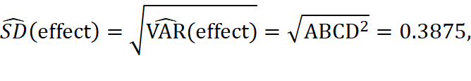
4-factor interactions |
0.3875 |
0.05 |
69.07 |
None |
|
|
3,4-factor interactions |
0.2577 |
0.05 |
1.23 |
A, B, D, AD |
|
|
2,3,4-factor interactions |
0.5505 |
0.05 |
1.64 |
A, B |
|
|
4-factor interactions |
0.3875 |
0.1 |
34.54 |
None |
|
|
3,4-factor interactions |
0.2577 |
0.1 |
1.04 |
A, B, D, AD |
|
|
2,3,4-factor interactions |
0.5505 |
0.1 |
1.43 |
A, B, D |
|
From the table, we can see that if only 4-factor interaction is negligible, no significance can be detected. If 3,4-factors interactions are negligible, effects A, B, D, and AD will be significant. If all 2,3,4-factor interactions are negligible, effects A and B will be significant at 95% level and effects A, B and D will be significant at 90% level.
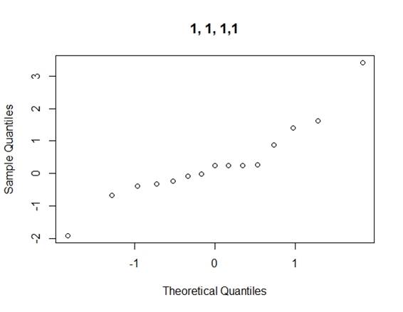
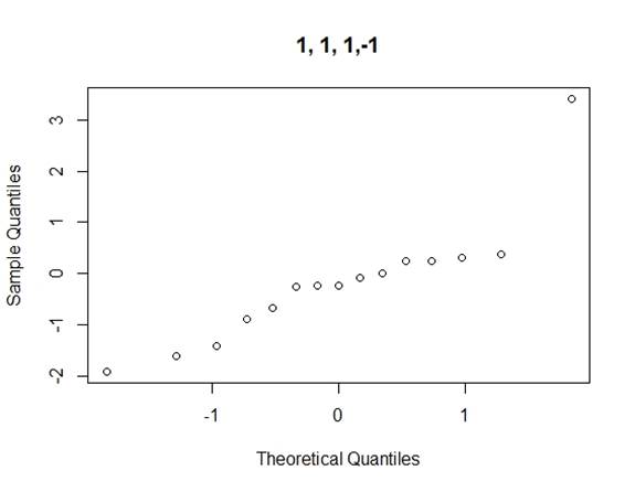
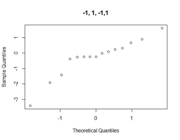
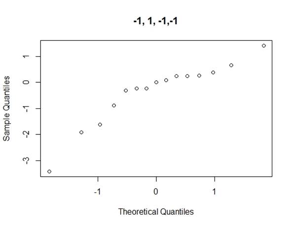
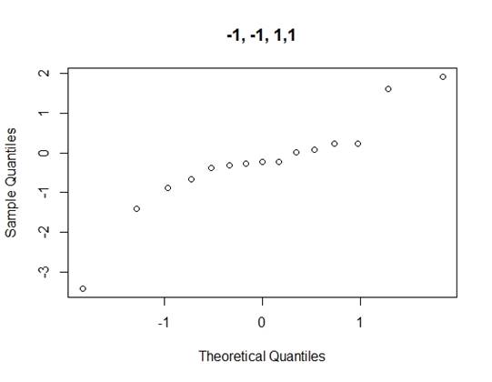
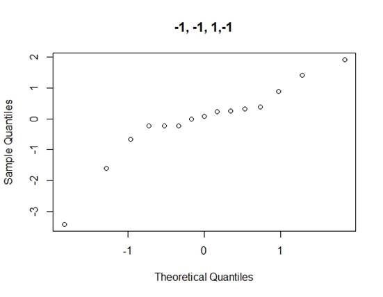
2.2.2 Loh��s Method
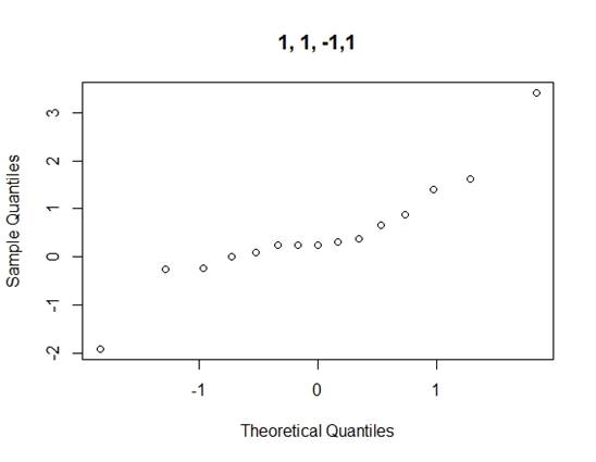
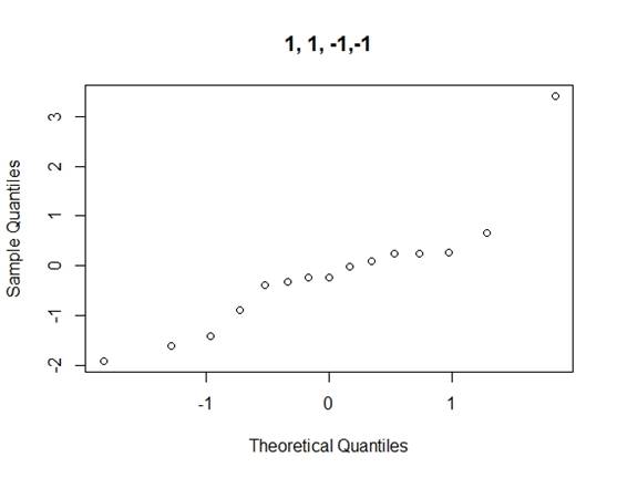
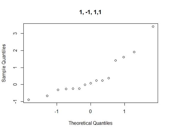
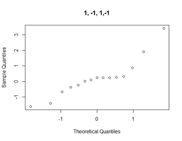
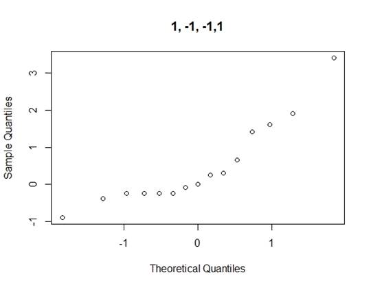
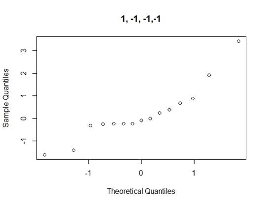
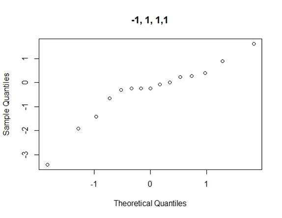
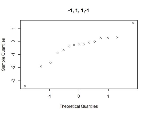
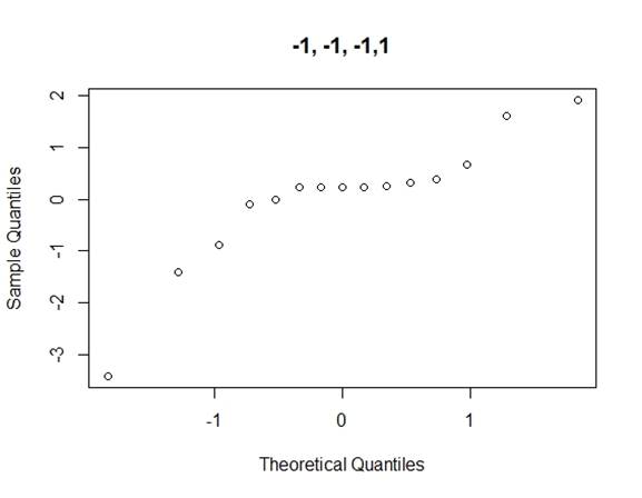
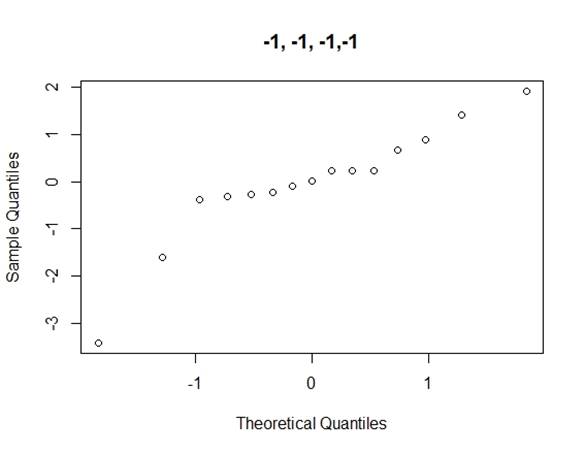
Considering the problems of Daniel��s method, we use Loh��s method (1992) to consider all normal qq-plots of estimated effects by switching factor labels (all plots can be found in the appendix) and choose the canonical plot with the lowest absolute value of median of the effects as follows (figure 2):
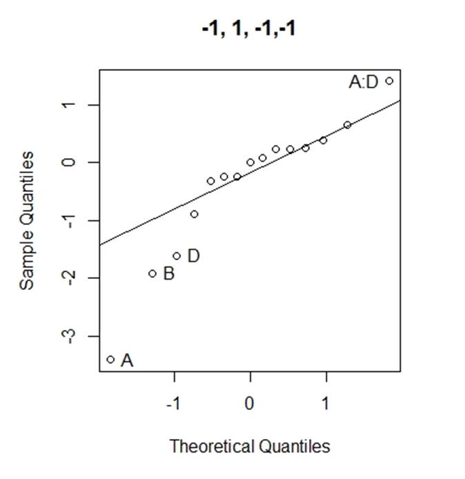
Figure 2: canonical qq-plot of effects
From the canonical qq-plot, it can be discovered that the effects A, B, D and AD looks like outliers, and thus these effects are significant.
2.2.3 Lenth��s Method
For Lenth��s method, for the set of effects ![]() , we first compute
, we first compute
![]()
and the pseudo standard error(PSE):
![]()
The margin of error (ME) is
![]()
and to avoid falsely identifying we also compute the simultaneous margin of error (SME)
![]()
where ![]() , and
, and ![]() . When
. When ![]() and
and
![]() , we can summarize the result we
got by the table 5:
, we can summarize the result we
got by the table 5:
Table 5: results of Lenth��s method at different level
|
|
ME |
SME |
Significant Effects |
|
0.05 |
0.9157698 |
1.8591445 |
A, B |
|
0.1 |
0.717861 |
1.568720 |
A, B, D |
Besides, we can also draw the Lenth plots (figure 3):
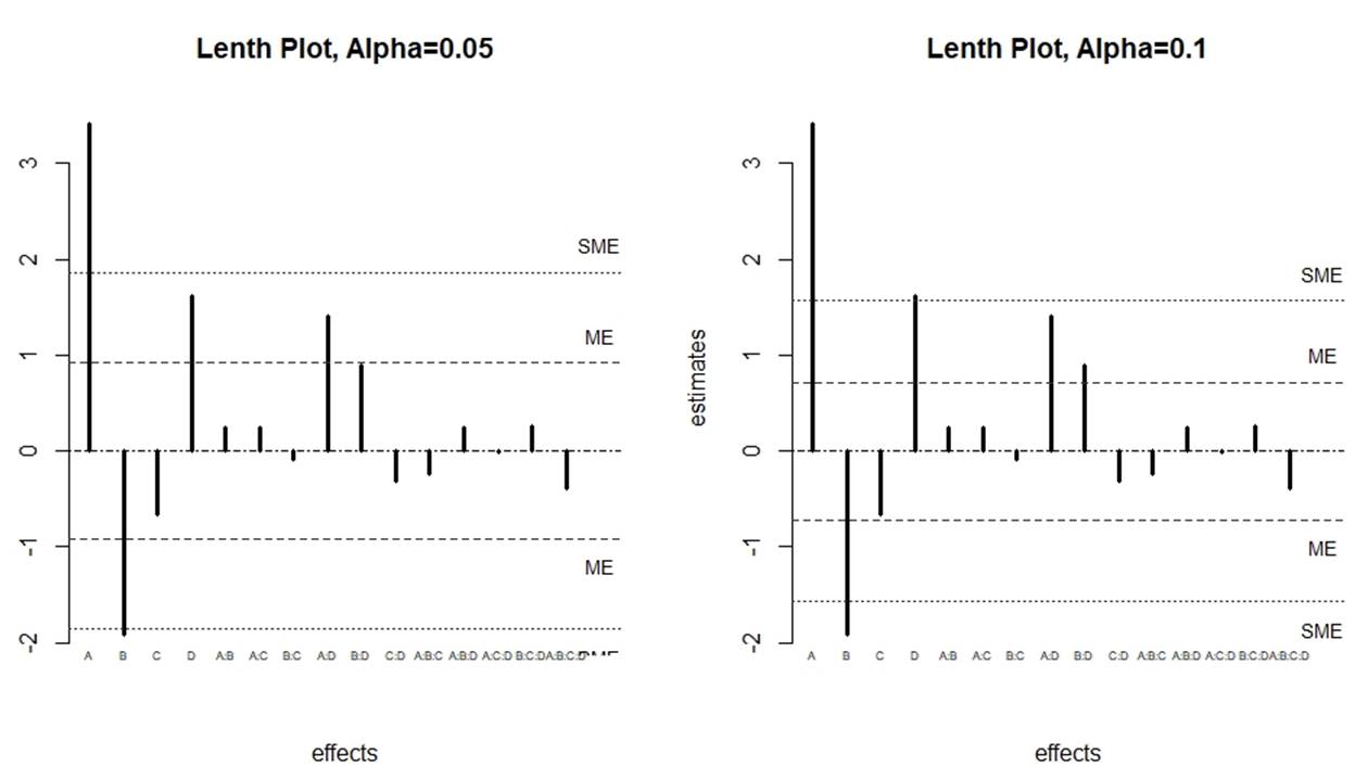
Figure 3: Lenth plots at different level
In the Lenth plot, x-axis stands for the effects, the y-axis stands for the corresponding estimates and the dash lines stand for the ME and SME.
From table 5 and figure 3, we can see that A and B are significant at 95% level, and A, B, and D are significant at 90% level. Additionally, it is notable that from the Lenth plot at 90% level, the effect AD is very close to SME, which means that it is also highly probable to be significant.
2.2.4 Dong��s Method
In Dong��s method, we first compute
![]()
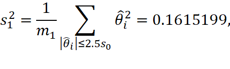
and
![]()
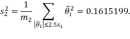
The simultaneous critical value is
![]()
where ![]() . When
. When ![]() ,
the critical value is 1.49288, and when
,
the critical value is 1.49288, and when ![]() , the critical value is 1.328783.
So, we can detect A, B, and D significant at 95% level and detect A, B, D and
AD significant at 90% level.
, the critical value is 1.328783.
So, we can detect A, B, and D significant at 95% level and detect A, B, D and
AD significant at 90% level.
2. 3 Conclusions
We have conclusions from both significance and methodology aspects:
Significance
We can summarize the results from the previous methods in the table 6 below:
Table 6: results of significance by different methods
|
Methods |
Levels |
Critical Value |
Significant Effects |
|
Estimate |
95% |
1.23 |
A, B, D, AD |
|
Loh��s method |
N/A |
N/A |
A, B, D, AD |
|
Lenth��s method |
95% |
1.86 |
A, B |
|
Lenth��s method |
90% |
1.57 |
A, B, D (candidate: AD) |
|
Dong��s method |
95% |
1.49 |
A, B, D |
|
Dong��s method |
90% |
1.33 |
A, B, D, AD |
From the table, we can see that all other methods can detect A, B and D at 90% level, and AD can also be a candidate for significant effects.
Methodology
Based on the dataset, it is easier for the neglecting high order interactions methods to detect significance, but it is possible that some important interactions may be neglected when using this method. Compared with Length��s method, Dong��s method can get a smaller critical value at the same confidence level, so Lenth��s method looks more conservative.
Additionally, when estimating variance by interactions, we can notice that if we only neglect 4-factor interactions, the critical value we get will be so big that none of the effects will be significant. This is because the degree of freedom used to estimate the variance is too small so that the result is unreliable.
3 Formal Experiment
After having the experience from the preliminary experiment, we can do the formal experiment. The data results and some related analysis are introduced in this section.
3. 1 Data Presentation
After another 5 days of formal experience, we collect and summarize the data in the table 7 below:
Table 7: data presentation of formal experiment
|
A |
B |
C |
D |
Replicates |
|
+ |
+ |
+ |
+ |
11.7, 10.3, 8.4, 8.6, 5.1, 4.8, 4.3, 8.2 |
|
+ |
+ |
+ |
- |
9, 4.5, 4.8, 3.5, 5.7, 3.4, 3, 2.2 |
|
+ |
+ |
- |
+ |
10.2, 12.3, 11, 11.8, 7.1, 8, 5, 5.3 |
|
+ |
+ |
- |
- |
7.9, 7.9, 7.3, 7.2, 3.6, 3.2, 4.5, 2 |
|
+ |
- |
+ |
+ |
12.8, 10.2, 8.1, 7.4, 9.6, 9.2, 9.1, 7.8 |
|
+ |
- |
+ |
- |
8.4, 8.7, 8.5, 7.2, 6.7, 5.9, 6.9, 5.8 |
|
+ |
- |
- |
+ |
11.4, 10.7, 11.7, 6.2, 7.9, 7.9, 7.8, 7.4 |
|
+ |
- |
- |
- |
9.2, 9.2, 7.9, 6.5, 7.4, 5.9, 5.8, 4.6 |
|
- |
+ |
+ |
+ |
6, 5.2, 2.4, 3.8, 0.4, 1.5, 0.2, 2.1 |
|
- |
+ |
+ |
- |
6.2, 1.9, 2.1, 0.4, 4.6, 0.4, 2.7, 2.2 |
|
- |
+ |
- |
+ |
4.6, 7.9, 5.6, 6.3, 4.6, 2.8, 1.4, 1.2 |
|
- |
+ |
- |
- |
3.5, 4.5, 6, 4.2, 2.1, 0.7, 0.8, 2.3 |
|
- |
- |
+ |
+ |
6.7, 6.8, 1.3, 3.8, 2.5, 4.6, 5.5, 3.1 |
|
- |
- |
+ |
- |
5.7, 6.1, 6.2, 5, 3.1, 2.1, 4.6, 3.6 |
|
- |
- |
- |
+ |
8.7, 6.2, 7.2, 4.4, 2.6, 5, 4.5, 4.1 |
|
- |
- |
- |
- |
6.7, 5.9, 7.3, 2.7, 4.8, 2.7, 2.9, 3.2 |
3. 2 Analysis of Variance
We have the full model
We can first estimate the effects as shown in table 8:
Table 8: effect estimates for the formal experiment
|
Effects |
Estimate |
Effects |
Estimate |
|
A |
3.4594 |
BD |
0.4500 |
|
B |
-1.5156 |
CD |
-0.2813 |
|
C |
-0.5719 |
ABC |
-0.2094 |
|
D |
1.5438 |
ABD |
0.2313 |
|
AB |
0.0156 |
ACD |
0.2750 |
|
AC |
0.1969 |
BCD |
-0.0625 |
|
BC |
-0.4656 |
ABCD |
-0.04375 |
|
AD |
1.0500 |
|
|
On 112 degrees of freedom, we can also compute the ![]() . Then, we can get the
simultaneous critical value
. Then, we can get the
simultaneous critical value
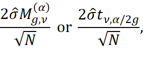
where ![]() , and
, and ![]() is the
is the ![]() quantile
of studentized maximum modulus distribution.
quantile
of studentized maximum modulus distribution.![]() . We also know that
. We also know that ![]() , which is very close to
, which is very close to ![]() . When
. When ![]() . The critical value means that
if the abstract value of an effect is greater than the critical value, this
effect will be significant at
. The critical value means that
if the abstract value of an effect is greater than the critical value, this
effect will be significant at ![]() level. So, we
can conclude the following table 9:
level. So, we
can conclude the following table 9:
Table 9: significance result
|
Distribution Used |
|
Critical Value |
Significant Effects |
|
Studentized Maximum Modulus |
0.1 |
1.005329 |
A, B, D, AD |
|
t-distribution |
0.1 |
1.008985 |
A, B, D, AD |
|
t-distribution |
0.05 |
1.096527 |
A, B, D |
The critical values of the two
distributions at same level are very close. This is because ![]() .
.
3. 3 Model Diagnosis
To make the results convincing, we need to check the assumptions of the models. In this subsection, we only check the normality and the equal variance assumptions.
3.3.1 Normality Check
To check the normalty, we draw the q-q plot of residuals (figure 4):
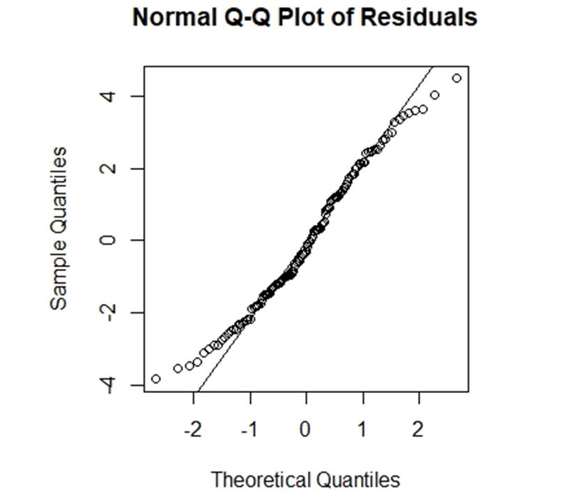
Figure 4: q-q plot of residuals
From figure 4, we cannot see any severe problem in this q-q plot.
3.3.2 Equal Variance Check
To check the equal variance, we draw the plot of residuals vs. fitted values (figure 5):
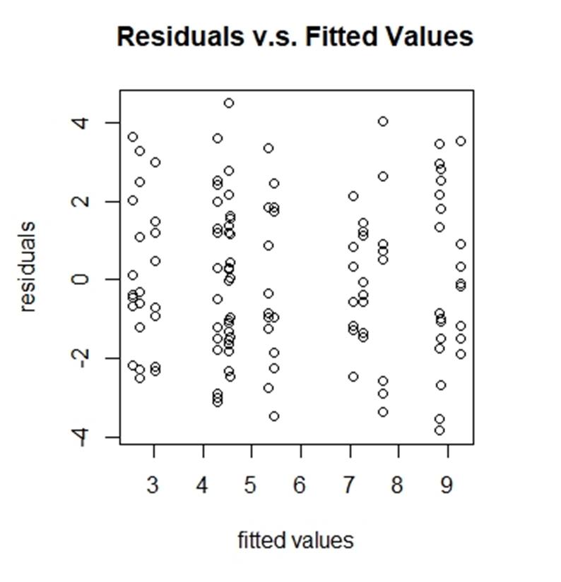
Figure 5: residuals vs. fitted values
From figure 5, we cannot see any severe unequal variance problem.
3.3.3 Cox-Box Transformation
Although the checking results of normality and equal variance looks not too bad, we still want to see what will happen if we do the cox-box transformation.
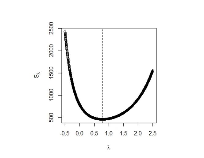
Figure 6:
![]() vs.
vs. ![]()
To get the best residual sum of squares ![]() , we choose
, we choose ![]() ,
do the transformation
,
do the transformation
![]()
and fit the new model again. We have the qq-plot and the residual vs. fitted value plot as follows
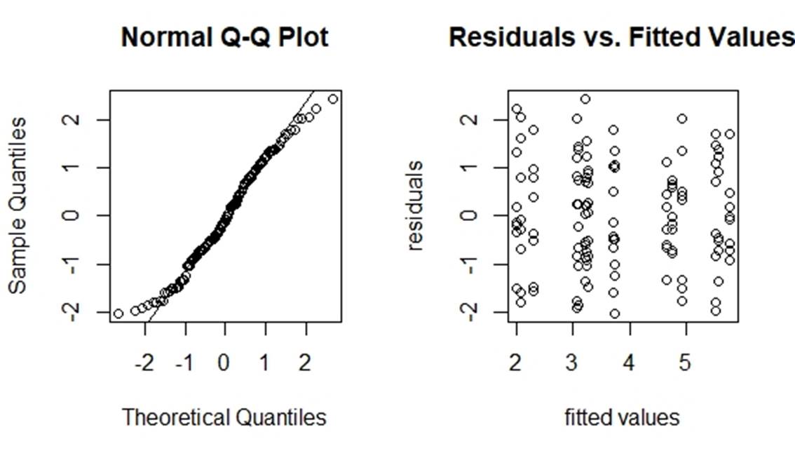
Figure 7: diagnosis of the transformed model
From figure 7, these two plots are not very different from those two from the original model. So, we think the transformation will not help too much. We can use the same method as stated in Section 3.2 to find the significant effects of the transformed model. After calculation, the result is still A, B and D.
3. 4 Final Model
The results from both preliminary and the formal experiment design indicates that effects A, B, D are significant at 95% level, and A:D is significant at 90% level. So, we have the final model 1:
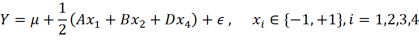
with the candidate model 2:
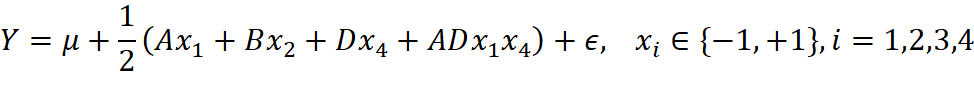
which is also highly possible to be a very good model.
3. 5 Fitted Values
For the full model, we can plug in the estimate and then have the fitted values as shown in the following table 10:
Table 10: fitted values for the full model
|
A |
B |
C |
D |
Fitted value (cm) |
|
+ |
+ |
+ |
+ |
7.7 |
|
+ |
+ |
+ |
- |
4.5 |
|
+ |
+ |
- |
+ |
8.8 |
|
+ |
+ |
- |
- |
5.5 |
|
+ |
- |
+ |
+ |
9.3 |
|
+ |
- |
+ |
- |
7.3 |
|
+ |
- |
- |
+ |
8.9 |
|
+ |
- |
- |
- |
7.1 |
|
- |
+ |
+ |
+ |
2.7 |
|
- |
+ |
+ |
- |
2.6 |
|
- |
+ |
- |
+ |
4.3 |
|
- |
+ |
- |
- |
3.0 |
|
- |
- |
+ |
+ |
4.3 |
|
- |
- |
+ |
- |
4.6 |
|
- |
- |
- |
+ |
5.3 |
|
- |
- |
- |
- |
4.5 |
For the good model 1 and model 2, we can also plug in the estimate and then have the fitted values as shown in the following table 10 and table 11:
Table 11: fitted values for model 1
|
A |
B |
D |
Fitted values (cm) |
|
+ |
+ |
+ |
7.4 |
|
+ |
+ |
- |
5.8 |
|
+ |
- |
+ |
8.9 |
|
+ |
- |
- |
7.4 |
|
- |
+ |
+ |
3.9 |
|
- |
+ |
- |
2.4 |
|
- |
- |
+ |
5.4 |
|
- |
- |
- |
3.9 |
Table 12: fitted values for model 2
|
A |
B |
D |
Fitted values (cm) |
|
+ |
+ |
+ |
7.9 |
|
+ |
+ |
- |
5.3 |
|
+ |
- |
+ |
9.4 |
|
+ |
- |
- |
6.8 |
|
- |
+ |
+ |
3.4 |
|
- |
+ |
- |
2.9 |
|
- |
- |
+ |
4.9 |
|
- |
- |
- |
4.4 |
4 Conclusions
Through this experiment, we discover that three of the main effects: A: Temperature, B: Impurity level of water and D: Watering frequency are significant while the interaction effect AD: between temperature and frequency is highly probable to be significant.
Since the estimates of the main effect A and D are positive and that of B is negative, it means that relatively higher temperature (25 Celsius) and higher watering frequency (every 6 hours) will accelerate the sprouting of the mung beans, while the high impurity level of water (Lake water) will restrain the sprouting.
The estimate of the interaction effect AD is also positive, and it means that if higher temperature and higher watering frequency are satisfied simultaneously, the sprouting speed will be improved additionally. This is possibly because that if the temperature is higher, the water from the mung beans will evaporate faster so that the need of water will become more essential.
The main effect C (soaking time) is found to be insignificant, which means that soaking mung beans for shorter time (6 hours) or longer time (12 hours) will not influence the sprouting speed too much. It is probable because after soaking in water for enough time and the mung beans beginning to sprout, superfluous water is not quite useful for the increasing sprouting speed.
References
Dong, F. (1993). On the identification of active contrasts in unreplicated. Statistica Sinica, 3:209-217.
Lenth, R. V. (1989). Quick and easy analysis of unreplicated factorials. Technometrics, 31:469�C473.
Loh, W.-Y. (1992). Identification of active contrasts in unreplicated factorial. Computational Statistics and Data Analysis, 14:135�C148.
Wu, C. F. (2000). Experiments: Planning, Analysis, and. Wiley.
Appendix
QQ-plots for Loh��s method
Code
library("MASS")
load('data.RData')
n=8
A = rep(c(rep(+1,16/2*n),rep(-1,16/2*n)),1)
B = rep(c(rep(+1,8/2*n),rep(-1,8/2*n)),2)
C = rep(c(rep(+1,4/2*n),rep(-1,4/2*n)),4)
D = rep(c(rep(+1,2/2*n),rep(-1,2/2*n)),8)
model = lm(Z~A*B*C*D)
anova = aov(Z~A*B*C*D)
anova(anova)
summary(model)
BoxCox = boxcox(Z~A*B*C*D,plotit = TRUE)
lambda = BoxCox$x[which.max(BoxCox$y)]
Znew = Z^lambda
model_trans = lm(Znew~A*B*C*D)
# ------------------------
n=1
A = rep(c(rep(+1,16/2*n),rep(-1,16/2*n)),1)
B = rep(c(rep(+1,8/2*n),rep(-1,8/2*n)),2)
C = rep(c(rep(+1,4/2*n),rep(-1,4/2*n)),4)
D = rep(c(rep(+1,2/2*n),rep(-1,2/2*n)),8)
# ------------------
modelpre = lm(Y0~A*B*C*D)
# --------------- Method 1
eff <- 2*modelpre$coefficients
sqrt(mean(eff[16:16]^2))*qt(0.05/2/14,df=1,lower.tail = F)
sqrt(mean(eff[12:16]^2))*qt(0.05/2/10,df=5,lower.tail = F)
sqrt(mean(eff[6:16]^2))*qt(0.05/2/4,df=11,lower.tail = F)
sqrt(mean(eff[16:16]^2))*qt(0.1/2/14,df=1,lower.tail = F)
sqrt(mean(eff[12:16]^2))*qt(0.1/2/10,df=5,lower.tail = F)
sqrt(mean(eff[6:16]^2))*qt(0.1/2/4,df=11,lower.tail = F)
# -- Lenth's Method
alpha=0.1
s0 <- 1.5*median(abs(eff))
PSE <- 1.5*median(abs(eff[abs(eff)<2.5*s0]))
ME <- PSE*qt(p = 1-alpha/2,df = (16-1)/3)
SME <- PSE*qt(p =(1+(1-alpha)^{1/15})/2,df=(16-1)/3)
library(BsMD)
par(mfrow=c(1,2),pty="s")
LenthPlot(modelpre,alpha=0.05,cex.fac = 0.5,xlab = 'effects', ylab='estimates',main="Lenth Plot, Alpha=0.05")
LenthPlot(modelpre,alpha=0.1,cex.fac = 0.5,xlab = 'effects', ylab='estimates',main="Lenth Plot, Alpha=0.1")
#---Dong's Method
efftemp = eff[2:16]
m1 = sum(abs(efftemp)<=(2.5*s0))
s1=sqrt(mean(efftemp[abs(efftemp)<=(2.5*s0)]^2))
m2 = sum(abs(efftemp)<=(2.5*s1))
s2=sqrt(mean(efftemp[abs(efftemp)<=(2.5*s1)]^2))
abs(eff)>(qt(p =(1+.95^(1/15))/2,df=m2,lower.tail = TRUE)*s2)
#---
alpha=0.05
r=8;k=4;g=2^k-1
N = 2^k*r
sigma=2.068
nu = 112
effects = 2*model$coefficients
t = 2*qt(alpha/2/g,df=nu,lower.tail = FALSE)*sigma/sqrt(N)
abs(effects)>t
n=8
A = rep(c(rep(+1,16/2*n),rep(-1,16/2*n)),1)
B = rep(c(rep(+1,8/2*n),rep(-1,8/2*n)),2)
C = rep(c(rep(+1,4/2*n),rep(-1,4/2*n)),4)
D = rep(c(rep(+1,2/2*n),rep(-1,2/2*n)),8)
# interaction.plot(A,D,Z)
par(mfrow=c(1,1),pty="s")
qqnorm(model$residuals,main = 'Normal Q-Q Plot of Residuals')
qqline(model$residuals)
plot(model$fitted.values,model$residuals,xlab = 'fitted values', ylab = 'residuals', main = 'Residuals vs. Fitted Values')
alpha=0.1
par(mfrow=c(1,2),pty="s")
model2 = lm(Z^lambda~A*B*C*D)
qqnorm(model2$residuals)
qqline(model2$residuals)
plot(model2$fitted.values,model2$residuals,xlab = 'fitted values', ylab = 'residuals', main = 'Residuals vs. Fitted Values')
effects2 = 2*model2$coefficients
sigma2=1.16
t2 = 2*qt(alpha/2/g,df=nu,lower.tail = FALSE)*sigma2/sqrt(N)
abs(effects2)>t2
# ----
par(mfrow=c(1,1),pty="s")
y0 <- Z ## yields in standard order
gm <- exp(mean(log(y0))) ## geometric mean
x1 <- A
x2 <- B
x3 <- C
x4 <- D
ssr <- NULL
lambda.seq <- seq(from=-0.5,to=2.5,length.out=1000)
for(lambda in lambda.seq){
if(lambda == 0){
y <- gm*log(y0)
} else {
y <- (y0^lambda-1)/(lambda * gm^{lambda-1})
}
fit <- lm(y ~ x1*x2*x3*x4)
ssr <- c(ssr,sum(fit$resid^2))
}
plot(lambda.seq,ssr,type="b",xlab=expression(lambda),
ylab=expression(S[lambda]))
abline(v=0.7878,lty=2)
# ------------
model1 = lm(Z~A+B+D)
fittedvalue1=c()
for(i in seq(1,121,8))
fittedvalue1 = c(fittedvalue1,round(model1$fitted.values,1)[i])
# -----------
model2 = lm(Z~A+B+D+A*D)
fittedvalue2=c()
for(i in seq(1,121,8))
fittedvalue2 = c(fittedvalue2,round(model2$fitted.values,1)[i])